
Mathematical Methods and Their Physical Implementation in Intensity-Modulated Radiation Therapy
Published:
Mathematical Methods and Their Physical Implementation in Intensity-Modulated Radiation Therapy
A Systematic Review Based on Inverse Planning (IMRT) and Multileaf Collimator Technology (MLC)
With advances in computer technology and mathematical optimization methods, Intensity-Modulated Radiation Therapy (IMRT) has become the core technique for dose-distribution control in modern radiation oncology. From the dual perspectives of mathematical modeling and physical implementation, this paper systematically reviews key technical developments in IMRT, focusing on analyzing inverse planning optimization, dynamic modulation by Multileaf Collimator (MLC), and the application of mathematical methods in clinical practice.
Mathematical Foundations of IMRT and the Principles of Inverse Planning
Mathematical comparison between forward planning and inverse planning
Conventional three-dimensional conformal radiotherapy (3D-CRT) uses a forward planning approach; its mathematical essence is a linear superposition model. Let the intensity distribution of the i-th beam be Ii, and the absorbed dose D(x) at point x in the patient can be expressed as:
\[D(x,y,z) = \sum_{i=1}^{N} \iint I_i(x',y') \cdot K(x-x', y-y', z) \, dx'dy'\]where K is the dose deposition kernel, describing the dose spread characteristics in tissue for a unit-intensity beam.
IMRT’s inverse planning converts the problem into a constrained optimization problem: given dose objectives for the target (PTV) D target D target Dose limits 𝐷 for organs at risk (OAR) OAR,max D OAR,max , solve for the optimal beamlet intensity distribution ${I_i}$ such that:
\[\begin{aligned} \text{Minimize} & \quad \sum_{j} w_j \left( D_j - D_{\text{target}} \right)^2 + \sum_{k} w_k \max\left( D_k - D_{\text{OAR,max}}, 0 \right) \\ \text{Requirement} & \quad I_i(x,y) \geq 0 \quad \forall i,x,y \end{aligned}\]Here 𝑤 𝑗 w j 与𝑤 k w k are weighting coefficients reflecting clinical priorities. The nonconvexity of this problem necessitates using iterative algorithms such as gradient descent or the simulated annealing algorithm to solve it.
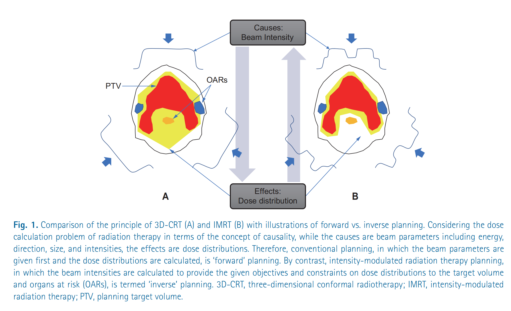
Illustration: Planning strategies of 3D-CRT vs. IMRT (forward vs. inverse)
This figure compares the principles of two radiotherapy planning approaches: three-dimensional conformal radiotherapy (3D-CRT) (A) and intensity-modulated radiotherapy (IMRT) (B), and uses the concept of causal relationships to illustrate the difference between forward planning and inverse planning.
Detailed explanation:
Overall structure of the figure: The figure connects “Causes: beam intensities” and “Effects: dose distribution” with a diamond-shaped structure. This diamond represents the causal relationship in a radiotherapy plan.
Figure A: 3D-CRT (forward planning):
- Causes: In 3D-CRT, beam parameters (energy, direction, size, intensity) are first determined. The figure uses simplified beam contour lines to represent the beams’ directions and shapes. Note that the beam intensities are usually uniform or vary little.
- Effects: Based on these beam parameters, the dose distribution is calculated. The red regions represent high-dose areas, and the yellow regions represent medium-dose areas. You can see that the high-dose regions largely cover the planned target volume (PTV), but also include parts of organs at risk (OARs). The arrow from “Causes” to “Effects” indicates the derivation from beam parameters to dose distribution, which is called “forward planning.”
Figure B: IMRT (inverse planning):
- Effects: In IMRT, the target dose distribution is determined first. That is, we want the planning target volume (PTV) to receive a sufficiently high dose while the organs at risk (OARs) receive as low a dose as possible.
- Causes: Then, the beam intensity distribution is derived by an optimization algorithm. The irregular beam contour lines in the figure represent the spatial variation of beam intensity in IMRT. It can be seen that, to achieve the desired dose distribution, the beam intensity in IMRT is nonuniform. The arrow from “Effects” to “Causes” indicates the process of back-calculating beam parameters from the dose distribution, which is called “inverse planning.”
Key concepts:
- PTV (Planning Target Volume): The planned target volume, i.e., the tumor region that needs to receive an adequate dose of radiation.
- OARs (Organs at Risk): Organs at risk, i.e., normal tissues or organs that should be spared from high-dose radiation as much as possible.
- Forward Planning: First determine beam parameters, then calculate the dose distribution.
- Inverse Planning: First define the dose distribution objectives, then derive the beam parameters.
Summary: This figure is intended to illustrate the fundamental difference in planning strategy between 3D-CRT and IMRT: 3D-CRT is a forward planning approach of “cause first, then effect,” whereas IMRT is an inverse planning approach of “specify the effect first, then find the cause.” The inverse planning of IMRT is better able to achieve complex dose distribution goals, thereby better sparing normal tissues and organs.
Analytical methods for dynamic modulation of the multileaf collimator (MLC)
What is multileaf collimator?
https://www.youtube.com/watch?v=msX1ypCjkK4
Kinematic model of the sliding window technique
The dynamic motion of MLC leaves must satisfy both dose-delivery and mechanical-motion requirements. Let the dwell time of a leaf pair at position $x$ be $t(x)$ ; then the cumulative dose $I(x)$ and the leaf velocity $v(x)$ can be modeled by:
\[\frac{dI}{dx} = \frac{dt}{dx} \cdot \dot{D} = \frac{\dot{D}}{v(x)}\]where $\dot{D}$ is the dose rate. For a given intensity distribution $I(x)$ , the Convery-Rosenbloom algorithm determines the dominant leaves by decomposing the sign of the gradient:
Convery-Rosenbloom algorithm: mathematical explanation
The Convery-Rosenbloom algorithm is a strategy for controlling the motion of multileaf collimator (MLC) leaves to achieve a target dose intensity distribution in intensity-modulated radiation therapy (IMRT). Its core idea is to dynamically adjust leaf speeds according to the gradient of the dose intensity distribution.
1. Symbol definitions:
x: spatial positionI(x): target dose intensity distributiondI/dx: gradient (rate of change) of the dose intensity distributionVmax: maximum leaf speedv1: Velocity of trailing leaf #1v2: Velocity of leading leaf #2
2. Algorithm rules:
The algorithm determines leaf velocities based on the following conditions:
Increase in dose intensity:
dI/dx > 0Leading leaf #2: moves at maximum speed.
v2 = VmaxTrailing leaf #1: speed depends on the rate of increase of dose intensity.
v1 = Vmax * (dI/dx) / (dI/dx)max; If the normalized gradient is usedHere
(dI/dx)maxrepresents the maximum gradient value that ensuresv1does not exceedVmax.
Dose intensity decrease:
dI/dx < 0Trailing leaf #1: moves at maximum speed.
v1 = VmaxLeading leaf #2: speed depends on the rate of dose intensity decrease.
v2 = Vmax * |(dI/dx)| / (dI/dx)max; If the normalized gradient is usedHere also
(dI/dx)maxis used to ensure a reasonable range for the speed.
Another equivalent expression (no normalization required):
Let $x_1(t)$ and $x_2(t)$ represent the positions of leaf 1 and leaf 2 at time t, respectively. Can be expressed as:
\[\begin{cases} v_2(t) = V_{max}, \quad v_1(t) = V_{max} \frac{\frac{dI}{dx}(x_2(t))}{\max_x \frac{dI}{dx}(x)} & \text{if } \frac{dI}{dx} > 0 \\ v_1(t) = V_{max}, \quad v_2(t) = V_{max} \frac{-\frac{dI}{dx}(x_1(t))}{\max_x (-\frac{dI}{dx}(x))} & \text{if } \frac{dI}{dx} < 0 \end{cases}\]Where $\max_x \frac{dI}{dx}(x)$ and $\max_x (-\frac{dI}{dx}(x))$ respectively represent the maximum rate of increase and the maximum rate of decrease of the dose intensity distribution gradient.
3. Core idea:
The Convery-Rosenbloom algorithm dynamically adjusts leaf speeds by analyzing the gradient of the dose intensity distribution, with the aims of:
- Maximizing efficiency: Ensuring at least one leaf moves at maximum speed to reduce treatment time.
- Physical feasibility: Avoiding instantaneous acceleration/deceleration of leaves to ensure smooth motion.
- Dose accuracy: Precisely shaping the dose intensity distribution to meet the treatment plan.
4. Summary:
The Convery-Rosenbloom algorithm achieves precise control of MLC leaf motion through simple rules. By intelligently adjusting leaf speeds, it realizes efficient, accurate dose modulation. When the target dose needs to increase, leading leaves quickly advance to “open the way,” while trailing leaves adjust their speeds as needed to “fill in”; when the target dose needs to decrease, trailing leaves quickly retreat to “close the door,” while leading leaves adjust their speeds as required.
- When $\frac{dI}{dx} > 0$ , the leading leaf moves at the maximum speed 𝑣 max v max Motion, trailing leaf speed $v_1 = v_{\max} \cdot \frac{I’(x)}{I’_{\max}}$
When $\frac{dI}{dx} < 0$ , the trailing leaf at 𝑣 max v max Motion, leading-leaf speed $v_2 = v_{\max} \cdot \frac{ I’(x) }{I’_{\max}}$
This method ensures the physical realizability of the leaf motion trajectories while minimizing the delivery time. The diagram below intuitively illustrates the geometric meaning of the algorithm through the time-space trajectories of leaf motion.
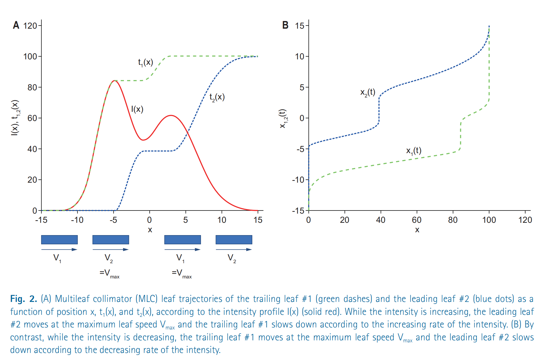
Diagram: Dynamic modulation of a multileaf collimator (MLC)
This figure shows how the multileaf collimator (MLC) dynamically adjusts leaf positions in intensity-modulated radiation therapy (IMRT) to achieve the desired dose intensity distribution. It is divided into two parts, A and B, which describe the motion of the MLC leaves from different perspectives.
Figure A
- Horizontal axis (x): represents spatial position.
- Vertical axis (I(x), t1,2(x)): represents dose intensity I(x) and the position functions t1(x) and t2(x) of leaf 1 and leaf 2.
- I(x) (red solid line): represents the desired dose intensity distribution. This curve shows the required dose intensity at different positions.
- t1(x) (green dashed line): represents the position of trailing leaf #1 as it varies with x.
- t2(x) (blue dotted line): represents the position of leading leaf #2 as a function of x.
- Arrows and V1, V2: show the direction of leaf velocities. When the intensity increases, leading leaf #2 moves at the maximum speed Vmax while the trailing leaf #1 slows down. Conversely, when the intensity decreases, trailing leaf #1 moves at the maximum speed Vmax while leading leaf #2 slows down.
The key point of Figure A is to explain how the Convery-Rosenbloom algorithm controls leaf velocities based on changes in the dose intensity distribution.
Figure B
- Horizontal axis (x): Still represents spatial position.
- Vertical axis (x1,2(t)): Represents the positions of leaf 1 and leaf 2 as functions of time t.
- x1(t) (green dashed line): The trajectory of the trailing leaf #1’s position over time.
- x2(t) (blue dotted line): The trajectory of the leading leaf #2’s position over time.
Figure B shows the evolution of leaf positions over time. It can be seen that the leaves do not move at a constant speed but accelerate or decelerate according to the requirements of the dose intensity distribution.
Summary
- Dose intensity distribution (I(x)) is the objective of the radiotherapy plan.
- Multileaf collimator (MLC) achieves this objective by adjusting the positions of the leaves.
- Convery-Rosenbloom algorithm is a strategy for controlling leaf motion that ensures the leading leaf moves at maximum speed when the dose intensity is increasing, while the trailing leaf moves at maximum speed when the dose intensity is decreasing. This effectively sculpts the dose distribution while ensuring physical feasibility.
- Leaf positions (x1(t), x2(t)) varying with time and space illustrate the entire dose modulation process.
Evolution of optimization algorithms in IMRT inverse planning
In inverse planning for intensity-modulated radiation therapy (IMRT), optimization algorithms are one of the core technologies. The following is a detailed explanation of algebraic iterative methods and quadratic programming, as well as mixed-integer programming based on dose–volume histograms (DVH).
1. Algebraic iterative methods
Background: Bortfeld and others likened the inverse problem of IMRT to the inverse Radon transform problem in CT image reconstruction. The goal of CT image reconstruction is to reconstruct the internal density distribution of an object from projection data, while the goal of IMRT inverse planning is to infer the beam intensity distribution from the desired dose distribution.
Formula: The update formula for the algebraic iterative method is:
\[I^{(n+1)} = I^{(n)} + \lambda A^T (D_{\text{prescribed}} - A I^{(n)})\]Where:
- $I^{(n)}$ : the beamlet intensity distribution at the $n$ th iteration.
- $A$ : the dose-influence matrix, describing each beamlet’s dose contribution to different voxels.
- D prescribed D prescribed : The expected dose distribution, i.e., the treatment objective.
- $A I^{(n)}$ : The actual dose distribution calculated under the current beam intensity distribution.
- $\lambda$ : Relaxation factor used to control the update step size.
Explanation:
- This method continuously adjusts the beam intensity $I^{(n)}$ so that the calculated actual dose $A I^{(n)}$ more closely matches the prescribed dose 𝐷 prescribed D prescribed 。
- The update direction is determined by residual $(D_{\text{prescribed}} - A I^{(n)})$ , and the residual is multiplied by $A^T$ to propagate into the beam intensity space.
- The relaxation factor $\lambda$ controls the update magnitude, preventing excessive adjustments that could cause instability.
Advantages and disadvantages:
- Advantages: Simple and intuitive, suitable for beginners to understand and implement.
- Disadvantages: Sensitive to noise and may lead to instability in the solution (such as oscillatory behavior).
2. Quadratic Programming
To overcome the shortcomings of algebraic iterative methods, IMRT optimization introduces a quadratic programming problem and adds a regularization term to suppress solution instability.
Formula:
\[\min_I \|A I - D_{\text{prescribed}}\|^2 + \alpha \|I\|^2\]Where:
- The first term $|A I - D_{\text{prescribed}}|^2$ : represents the sum of squared errors between the actual dose and the target dose, called the data fidelity term.
- Second term $\alpha |I|^2$ : the regularization term, used to limit the magnitude of beam intensities $I$ and prevent excessive intensity fluctuations.
- $\alpha$ : the regularization parameter that controls the trade-off between the data-fitting term and the regularization term.
Explanation:
- Quadratic programming minimizes both dose error and beam-intensity instability simultaneously by optimizing an objective function.
- The regularization term (also called Tikhonov regularization) can suppress the effect of noise on the solution, making the optimization results smoother and more stable.
Advantages and disadvantages:
- Advantages: More stable compared to algebraic iterative methods and not sensitive to noise.
- Disadvantages: Requires more computational resources to solve the quadratic programming problem.
3. Mixed-integer programming based on DVH (dose–volume histogram)
Background: In clinical practice, physicians typically use the DVH to evaluate whether a treatment plan meets the requirements. For example:
- Target volume (PTV): a certain proportion of the volume needs to reach the prescribed dose.
- Organs at risk (OAR): A specified proportion of the volume must be kept below a certain dose threshold (for example, “V20 < 30%” means the volume receiving less than 20 Gy must be under 30%).
To satisfy these nonlinear constraint conditions, they can be transformed into a mixed-integer programming problem.
Formula:
\[\sum_{m=1}^{M} \theta_m \cdot V_m \leq V_{\text{limit}}, \quad \theta_m \in \{0,1\}\]Where:
- $M$ : total number of voxels.
- V m V m : Volume corresponding to voxel $m$ .
- 𝜃 𝑚 θ m : A binary variable indicating whether the $m$ th voxel exceeds the threshold dose (1 means exceeds, 0 means does not exceed).
- V limit V limit : Maximum volume allowed under the constraints.
Explanation:
- By introducing the binary variable 𝜃 m θ m convert DVH constraints into linear or piecewise-linear constraints so they can be incorporated into the optimization framework.
- Mixed-integer programming problems include continuous variables (such as beam intensities) and discrete variables (such as 𝜃 𝑚 θ m ), so the problem is relatively difficult to solve.
Solution method: Because mixed-integer programming is computationally complex, the following methods are usually used for approximate solutions:
- Heuristic algorithms (such as genetic algorithms and simulated annealing).
- Branch-and-bound methods or relaxation techniques.
Summary
- Algebraic iterative methods: Simple and fast but sensitive to noise, suitable for preliminary optimization.
- Quadratic programming: Introduces regularization terms to suppress noise, more stable, but with higher computational complexity.
- Mixed-integer programming: Used to satisfy clinical DVH constraints, converting complex nonlinear conditions into linear constraints, but difficult to solve and often requires heuristic algorithms.
These methods together form the optimization algorithm framework in IMRT inverse planning, progressively increasing accuracy and clinical feasibility from simple to complex.
Application Cases
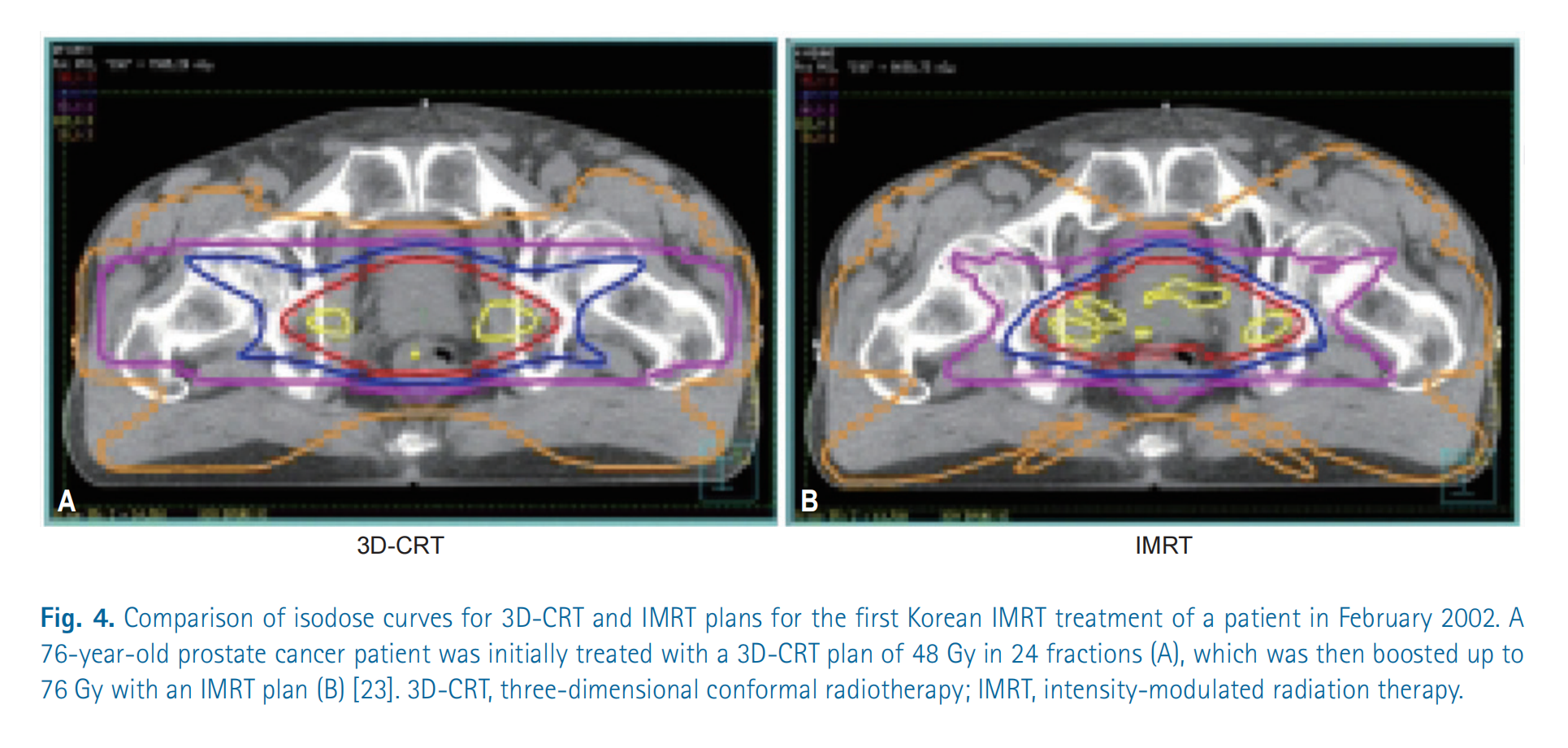
Illustration: 3D-CRT vs. IMRT Dose Distribution
This figure compares two radiotherapy plans: three-dimensional conformal radiation therapy (3D-CRT) and intensity-modulated radiation therapy (IMRT). The purpose is to show the differences in dose distribution between the two methods for the treatment of prostate cancer.
Detailed Explanation:
CT scan images: Both images are cross-sections of CT scans of the patient’s pelvic region. The pelvis, soft tissues, and the location of the prostate can be seen.
Isodose Curves: The curves marked in different colors in the figure represent isodose lines. Isodose lines connect points receiving the same radiation dose.
- Different colors represent different dose levels.
Figure A: 3D-CRT plan:
- The isodose lines appear relatively regular, forming concentric circles or ellipses.
- The high-dose region (usually shown in red or yellow) is mainly concentrated in the prostate area, but it also covers a larger amount of the surrounding tissue. This means that nearby normal tissues are also exposed to higher radiation doses.
- Overall, 3D-CRT can adequately cover the target area, but its protection of surrounding tissues is relatively poor.
Figure B: IMRT plan:
- Isodose lines are irregularly shaped, allowing better conformity to the shape of the prostate.
- High-dose regions are more concentrated in the prostate area, and surrounding normal tissues receive significantly reduced radiation.
- IMRT technology can achieve a more precise dose distribution by modulating beam intensities, thereby better protecting surrounding healthy tissues while ensuring the tumor receives the prescribed dose.
Summary:
- This figure clearly demonstrates the advantages of IMRT over 3D-CRT: better dose conformity, the ability to more precisely concentrate high doses on the tumor region, and reduced damage to surrounding healthy tissues.
- This means IMRT treatment plans can typically reduce side effects and improve patients’ quality of life.
Direct aperture optimization and rotational irradiation techniques
1. Direct Aperture Optimization (DAO)
Background: In IMRT, the aperture shapes of the MLC (multileaf collimator) and the beam weights need to be optimized to achieve the desired dose distribution. Traditional methods typically proceed in two steps:
- Optimize the beam intensity distribution.
- Generate MLC leaf sequences based on the optimization results.
Direct aperture optimization (DAO) combines these two steps by directly optimizing MLC aperture shapes and beam weights. Because aperture shapes are discrete variables, the entire optimization problem falls into the category of discrete combinatorial optimization problems.
Application of genetic algorithms:
Shepard et al. proposed using a genetic algorithm to solve the DAO problem. Genetic algorithms are heuristic search methods based on the principles of natural selection and genetics, particularly well suited to solving complex combinatorial optimization problems.
Genetic algorithm steps:
Initialize the population:
- Randomly generate $N$ feasible MLC aperture sets; each individual represents a possible solution.
- Each individual contains a set of MLC leaf positions and the corresponding beam weights.
Fitness evaluation:
- Compute the objective function value for each individual.
The objective function typically includes the following parts:
\[f = w_1 \cdot \text{Dosage error} + w_2 \cdot \text{Machine Unit (MU)}\]Where:
- Dose error: Represents the discrepancy between the actual dose distribution and the target dose distribution.
- Monitor Unit (MU): Represents the total beam intensity required for the treatment, reflecting treatment efficiency.
Selection:
- Sort by fitness values and retain the top 50% of individuals for the next generation.
Crossover:
- Randomly select two individuals and exchange part of their aperture information to generate new offspring.
- For example, swap a portion of the MLC leaf sequences between two individuals.
Mutation:
- With probability $p$ randomly adjust the aperture boundaries or beam weights of certain individuals.
- The goal is to introduce diversity and prevent getting trapped in local optima.
Results and advantages:
- In prostate cancer cases, compared with the conventional two-stage method, DAO reduced machine units (MU) by about 15%, improving treatment efficiency.
- Genetic algorithms, by simulating the process of natural evolution, can find solutions close to the global optimum in complex solution spaces.
2. Volumetric Modulated Arc Therapy, VMAT
Background: VMAT is an extended form of IMRT that allows radiotherapy equipment to dynamically adjust beam intensity, MLC leaf positions, and dose rate during continuous rotation. This approach greatly improves treatment efficiency while maintaining high-quality dose distributions.
Mathematical modeling:
The optimization problem for VMAT can be described using optimal control theory:
\[\min_{u(t)} \int_{0}^{T} L(\mathbf{x}(t), u(t)) \, dt\]Where:
- $T$ : treatment time (i.e., the time required for the device to complete one rotation).
- $L(\mathbf{x}(t), u(t))$ : objective function, representing the quality of the treatment plan, including dose errors and machine parameter variations.
- $\mathbf{x}(t)$ : state variables, including:
- Cumulative dose distribution at points within the patient’s body.
- Mechanical parameters of the treatment device (such as gantry angle, MLC leaf positions, dose rate).
- $u(t)$ : control inputs, including:
- MLC leaf speed.
- Beam dose-rate variation.
Solution method:
Adjoint method for computing gradients:
- Use the adjoint equation to compute the gradient of the objective function with respect to the control input $u(t)$ .
- Gradient information is used to guide the optimization direction so that the objective function decreases progressively.
Sequential Quadratic Programming (SQP):
- Decomposes the nonlinear optimal control problem into a series of quadratic programming subproblems.
- At each iteration, a quadratic programming problem is approximately solved and the control input $u(t)$ is updated.
Results and Advantages:
- VMAT achieves more efficient and more precise treatment plans by delivering radiation through continuous rotational irradiation.
- Compared with conventional IMRT, VMAT significantly reduces treatment time while maintaining good target coverage and sparing of normal tissues.
Conclusion
Direct Aperture Optimization (DAO):
- Jointly optimizing MLC aperture shapes and beam weights is a discrete combinatorial optimization problem.
- Genetic algorithms efficiently search complex solution spaces by simulating the process of natural selection, significantly improving treatment efficiency.
Volumetric Modulated Arc Therapy (VMAT):
- Based on optimal control theory, continuously rotating irradiation is achieved by dynamically adjusting device parameters.
- The adjoint method and SQP algorithm are used to solve it, shortening treatment time while ensuring high-quality dose distribution.
Monte Carlo methods and GPU acceleration in dose calculation
Supplementary Monte Carlo simulations
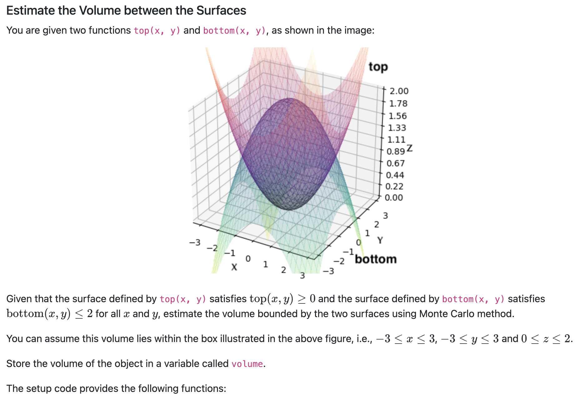
| Name | Type | Description |
|---|---|---|
| top | function | Returning the z coordinate given (x, y) for the function on the top |
| bottom | function | Returning the z coordinate given (x, y) for the function at the bottom |
Your code snippet should define the following variable:
| Name | Type | Description |
|---|---|---|
| volume | float | The estimated volume of the object as described in the question |
Solution code:
import numpy as np

# Define bounding box limits
x_min, x_max = -3, 3
y_min, y_max = -3, 3
z_min, z_max = 0, 2

# Number of random samples
N = 1000000

# Calculate bounding box volume
bounding_box_volume = (x_max - x_min) * (y_max - y_min) * (z_max - z_min)

# Generate random samples within the bounding box
x_samples = np.random.uniform(x_min, x_max, N)
y_samples = np.random.uniform(y_min, y_max, N)
z_samples = np.random.uniform(z_min, z_max, N)

# Evaluate top and bottom surfaces at sampled (x, y) points
top_values = np.array([top(x, y) for x, y in zip(x_samples, y_samples)])
bottom_values = np.array([bottom(x, y) for x, y in zip(x_samples, y_samples)])

# Check if points lie between bottom and top surfaces
valid_points = (z_samples >= top_values) & (z_samples <= bottom_values)

# Estimate volume as fraction of valid points multiplied by bounding box volume
volume_fraction = np.sum(valid_points) / N
volume = volume_fraction * bounding_box_volume
GPU-based parallel dose engine
Modern IMRT planning systems use GPU-accelerated Monte Carlo algorithms, with the following thread allocation strategy:
- Each thread block processes one beam
- Each thread simulates $10^4$ photon histories
- Use atomic operations to update voxel dose
Compared with the CPU version, the GTX 1080 Ti can achieve a $200\times$ speedup, making the Monte Carlo algorithm clinically practical.
Multi-objective optimization and Pareto frontier analysis
Parametric representation of the Pareto solution set
A multi-objective optimization problem can be represented as:
\[\min_{\mathbf{x}} \left( f_1(\mathbf{x}), f_2(\mathbf{x}), ..., f_k(\mathbf{x}) \right)\]Monz and others proposed the strong>normal vector method to parametrize the Pareto frontier:
\[\mathbf{w} = \frac{\nabla f_i}{\|\nabla f_i\|}, \quad \alpha = \arccos(\mathbf{w}_i \cdot \mathbf{w}_j)\]By interactively adjusting the weight vector $\mathbf{w}$ , clinicians can intuitively explore the trade-off between target coverage and OAR protection.
Statistical process control in quality assurance
Dose verification analysis based on control charts
Pawlicki proposed incorporating IMRT QA results into the statistical process control system:
- Calculate the mean $\mu$ and standard deviation $\sigma$ of historical data
- Define control limits: $\mu \pm 3\sigma$
- Perform root cause analysis on cases that exceed the control limits
This method reduced the QA failure rate from 12% to 4%, while also reducing measurement workload by 30%.
Future development direction: artificial intelligence and adaptive radiation therapy
Application of deep learning in inverse planning
Recent studies have attempted to use convolutional neural networks (CNNs) to directly map CT images to optimal beam intensities:
\[I = \text{CNN}(CT, PTV, OARs; \theta)\]where $\theta$ denotes the network parameters. Preliminary results show that for prostate cancer cases, inference time can be reduced to 5 seconds, and the dose distribution pass rate exceeds 90%.
Conclusion
The history of IMRT development is essentially a paradigm of collaborative innovation between mathematical modeling and engineering technology. From Brahme’s analytical solutions to the inverse problem to modern deep-learning–assisted planning, innovations in mathematical methods have continuously driven improvements in radiotherapy accuracy. As multi-physics coupled models and real-time adaptive optimization algorithms advance, IMRT will play an increasingly central role in personalized cancer treatment.
Reference
Bao, P., Wang, G., Yang, R., & Dong, B. (2023). Deep Reinforcement Learning for Beam Angle Optimization of Intensity-Modulated Radiation Therapy. arXiv preprint arXiv:2303.03812.
Cho B. Intensity-modulated radiation therapy: a review with a physics perspective. Radiat Oncol J. 2018 Mar;36(1):1-10. doi: 10.3857/roj.2018.00122. Epub 2018 Mar 30. Erratum in: Radiat Oncol J. 2018 Jun;36(2):171. doi: 10.3857/roj.2018.00122.e1. PMID: 29621869; PMCID: PMC5903356.
Moreau, G., François-Lavet, V., Desbordes, P., & Macq, B. (2021). Reinforcement learning for radiotherapy dose fractioning automation. Biomedicines, 9(2), 214